Optical Music Recognition | Alexander Pacha

Optical Music Recognition – A Beginners Guide

Posted on January 6, 2024January 6, 2024 by apacha

I’m regularly receiving e-mail from people all around the world that discovered the fascinating research field of Optical Music Recognition (OMR), the field that studies how to computationally read music notation in documents. I’ve decided to collect some answers here about questions that I usually get asked to provide you with a smoother journey into this field.

What is Optical Music Recognition?

This scientific article gives a thorough introduction, but frankly speaking, I understand if you don’t want to read 30 pages, so here’s the gist: With Optical Music Recognition we try to build computer programs that can make some sense out of notated music (typically printed on paper) like this, ideally enough to allow us to do nice things with it:

For example, play it back to us, that we get a feeling of how the music sounds like.

Or maybe even give us the entire music in a format that allows us to edit it in a music score editor like MuseScore.

MuseScore Representation of the Music Download

Depending on what we want to achieve, the computer needs to comprehend more or less:

If we just want to understand whether there is some music in an image or not, we don’t need very complicated methods. But if we want to reconstruct everything we need to find and understand everything that appears in an image. While the ultimate goal would be to build a system that can obtain the structured encoding (e.g., a MusicXML file), you can already enable many useful application with a simpler system.

How does Optical Music Recognition relate to other fields and how is it different from Optical Character Recognition?

OMR overlaps with several other fields, and heavily relies on computer vision methods to visually understand the content of an image:

However, OMR is expected to not just visually understand the contents of an image, but also restore the underlying music (at least to a certain degree). Simply put: It’s not enough to just find the dots and lines in this image, but we also have to understand what they mean and that depending on where dots appears, they mean something completely different:

Three quarter notes with dots. The first one is a dotted quarter, which extends the duration, the second one is a staccato note, which (broadly speaking) shortens the duration. The third one has both a staccato articulation and a duration dot. How to correctly perform this can be tricky 😅.

Music notation is a featural writing system, which makes it different from written text. A black dot in music notation means nothing on it’s own. Only the configuration—how they are placed in relation to other objects—give it meaning. What the exact meaning is, is defined by the syntactic and semantic rules of music notation.

Why is Optical Music Recognition hard?

There are a couple of reasons, why OMR is considered a very hard challenge and until this day is subject to ongoing research.

Visual Recognition

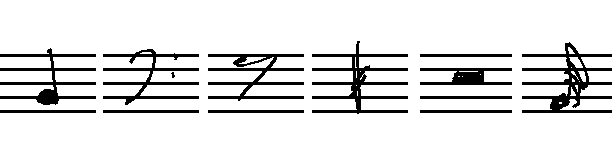
For beautifully written and typeset music sheets, this seems to be an easy task with modern computers, but when it comes to handwritten music, even humans sometimes struggle to make some sense out of the music:

Errors propagate

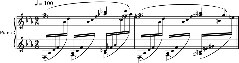
Tiny errors can have catastrophic consequences: Consider this small snippet of Debussy’s Clair de Lune:

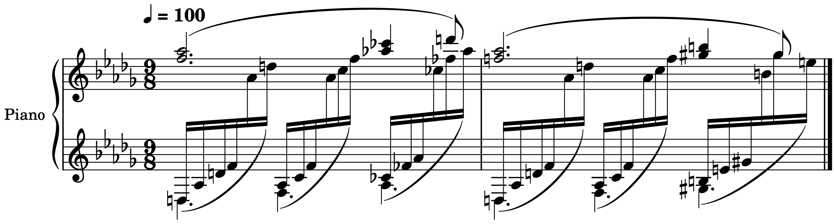
If we just miss two tiny accidentals at the beginning, the result is completely different:

Such small errors can be the results of image degradations and while the computer managed to correctly recognize 99% of all symbols, the result can still be so bad, that musicians are unwilling to accept the result, because they rely on the correctness of the score to perform a piece of music.

Correcting errors is non-trivial

The support for correcting errors in common music notation editors is not great, because they were not built for it. Say, if I want to fix the error from above by changing the key signature again, MuseScore will automatically generate a couple of accidentals to keep the pitch of all notes the same. So we fixed one problem, but introduced many others:

The rules of music notation are sometimes bent (or even broken)

Musicians are expected to not only be able to read music scores, but also have a profound understanding of the rules that govern it. It’s a process that can take years, and even then you will still encounter situations that will make you wonder, what the intention of the composer was. One common example of violated rules of music notation is the meter in music that has many triplets:

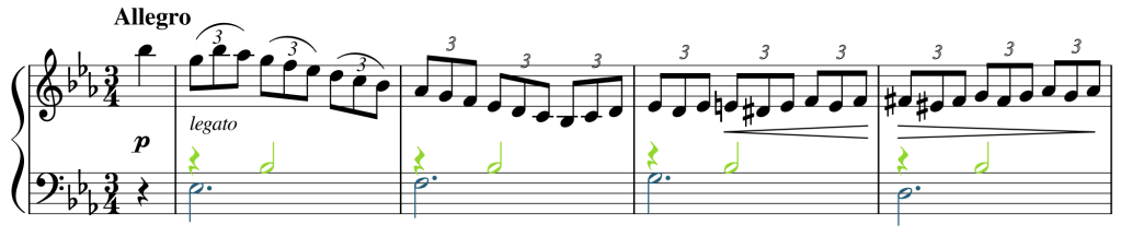
This visualization includes all triplets, but the small 3 on top of the eighth notes are commonly omitted, starting with the second bar. If you were to be a computer that strictly interprets the durations of the notes as they appear, this would cause problems, because you now have 9 eighth notes in a measure where you only expect 6, which violates the meter of the measure.

In some extreme examples, ambiguities and violations of the rules of music notation leave us no choice but to evaluate different hypotheses and pick the most likely one.

*In this example the dot in the red box could be associated with two different noteheads (only one makes sense). And the measure in the green box has one sixteenth note too much for the given meter.*

How does Optical Music Recognition work?

Over the past 50 years, many researchers attempted to build systems that are capable of reconstructing music from images. Most approaches use a pipeline to process images, similar to this one:

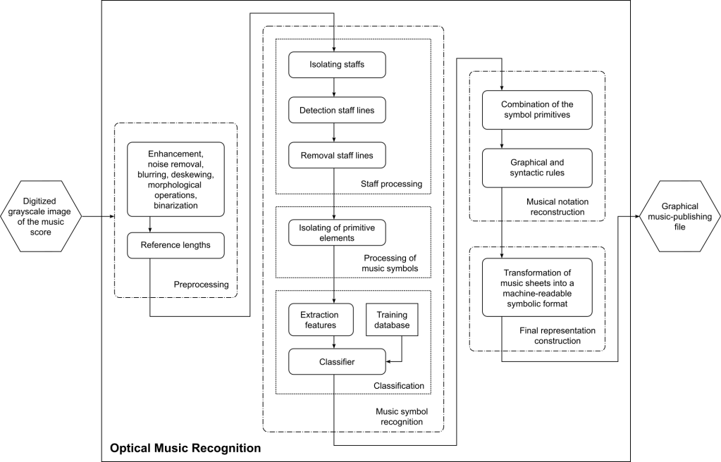
With the advent of Deep Learning, some steps have been merged, removed, or added, but most approaches still build upon the idea to perform one step after another, trying to recover more and more information as they move along.

The most notable exception to this rule are so-called end-to-end systems, that try to use a machine-learning approach that performs all these steps in a single neural network. While such approaches are still limited, they are an appealing alternative to explore in the future.

I want to build an Optical Music Recognition system myself – how do I start?

Depending on where you come from, I recommend you to familiarize yourself with the following things:

Music notation: Especially if you are an engineer, you might not be familiar with all of the intricacies of music notation and underestimate the complexity. Seeing simple examples is quite different from experiencing more interesting music notation in the wild. A system that only works for a small toy example is simply not sufficient. Not even for Mozart.
Deep Learning: Machine learning, especially deep learning, has fueled most of the advances the field made in the last 5-10 years. If you have no knowledge about deep learning, you’re in luck, because I’m teaching it at the TU Wien and you can watch all of my lectures on YouTube. If you prefer to read instead, there are also plenty of textbooks available.
Terminology of the field: If you are really serious about your research, you need to familiarize yourself with the terminology, taxonomy, and goals. Now would be a good time to do read this scientific article.
Define your own goals: Once you understand OMR to a certain degree, think about your own goals. What do you want to achieve with it? What is the problem you’re trying to solve? Why is it a problem? What would be your solution and why is it a solution? Which resources do you have? Don’t underestimate the complexity of this field. Having a few months for a master thesis will allow you to tackle one small (sub-)problem, but will not allow you to build an entire OMR system from scratch.
State-of-the-art and open questions: Once you go into research, you need to be aware of what is going on in the field. Hundreds of scientific articles have been published so far. Most of them are listed in the OMR Research Bibliography. Study the recently published articles, attend workshops and conferences and connect with fellow researchers. Maybe you can collaborate with someone, who is interested in doing the same thing.

If you have completed the steps from above and still have questions, feel free to contact me. Good luck with your research!

Recording of Doctoral Defense

Posted on July 5, 2019July 21, 2019 by apacha

I am very happy to announce that I’ve successfully completed my doctoral studies and defended my thesis on the 4th of July 2019. I’m now officially Dr. techn. Alexander Pacha.

For my defense, I prepared a 45-minutes presentation. Unfortunately, not everyone who might be interested in it was able to physically join the event, so I decided to re-record the presentation and uploaded the video to YouTube. I hope you enjoy watching it, as it summarized all of the work that I’ve been doing in the last two-and-a-half years in less than an hour:

The icon used as featured image was made by Icon Pond from www.flaticon.com and is licensed under CC 3.0 BY license.

From an infant to a toddler – how my computer learnt to detect music symbols

Posted on April 9, 2018May 16, 2018 by apacha

In my last post on optical music recognition, my computer was an infant. It was merely able to utter words if presented with an isolated image of a single object. It could distinguish a quarter rest from a g-clef, similar to a baby that can distinguish an apple from a banana. Nothing more. But, it learnt all that by itself (!), only given a couple of thousand annotated examples and a powerful PC.

In this post, I am proud to announce, that my machine has grown up and is now a toddler. It still can’t run or talk. But it can crawl around and find all apples and bananas in the room. It is now capable of detecting music symbols in the music scores like this:

It’s hard to see anything, right? Well, that’s because there are a lot of things going on in music scores. But let’s take it step by step.

If you haven’t read my previous post or following my research, here is the TL;DR: I am teaching my computer to read music scores to do such cool stuff as listening to scores, after taking a picture of them with your smartphone. But while the idea is not new at all, I am following a radically new approach and instead of telling (programming) the computer what to do (first look for lines, then for round objects, then combine them, …), I am letting the computer figure that out by itself. The whole thing is a five-step process, described here, of which I am currently working on step number three: detecting music objects.

We are using deep learning techniques, where a big (convolutional) neural network (think of it as something, that tries to imitate how the brain works) is being shown thousands of images like the following one, along with the information, what is in there and watch what happens over time:

While it starts with only a limited number of simple symbols, that are being detected, it quickly figures out how to detect all sorts of symbols. And while it is clearly not perfect, e.g. the half rest is confused with a whole rest in the above stave, it is remarkable, what the network was capable of learning by itself. If you are interested in the technical details, they are described in a scientific paper, that I will present at this year’s International Workshop on Document Analysis Systems in Vienna. But to summarize it: The computer scans the image along a grid with predefined “boxes” and evaluates each box, on whether it contains something of interest or not, called “objectness score”. Once, it found all (or most) potential boxes, it starts to refine them and assign a label to each box, e.g. “I think that is a G-clef in the left upper corner at position X, Y”. This process is end-to-end trainable with the so-called Faster R-CNN approach and was implemented with Tensorflow’s Object Detection API.

Did you notice, that the scores here were handwritten? That’s right. We are working on the CVC-MUSCIMA dataset that contains 1000 handwritten music scores, which was annotated in the MUSCIMA++ dataset by my outstanding colleague Jan Hajič, whose effort I am very grateful for.

And while this looks nice already, it has one significant drawback: The images you see above are not the entire score. What happens to a symbol that is bigger than image section? Well, it is not detected at the moment. But I wouldn’t mention it here if that was the end of the line. In fact, I’ve been working on detecting symbols in the full image already, and the first results are very promising:

It still has a couple of other issues, for example some very small objects, that were not properly detected or some confusions, but it is already a big step towards making this work in such a way, that the computer will be able to improve over time, by simply providing more data.

I will continue to work on the object detection a little longer before I start teaching the computer, what those symbols actually mean. Once I taught him how to find the symbols, how they relate to each other and what they mean, I hope it will grow up and sing beautiful songs to me. Until then, I will have to sing them by myself. 🙂

Update 27.04.2018: If you are interested, here is my presentation on this subject, that I gave at the DAS 2018.

Aligning images – an engineer’s solution

Posted on January 29, 2018March 24, 2019 by apacha

Recently I was struggling with the fact that one of the datasets, that I was working with had the same images, but they were not correctly aligned. Since one of them had location annotations that I used for training a Music Object Detector, I had to align them somehow.

For getting an impression on the alignment-error, look at the following images:

Black-and-White Image

Unaligned Grayscale Image

Bitwise difference between the images

The top-left image is the binarized image which serves as a reference. The top-right image is the original gray-scale image that is misaligned a tiny little bit, which you can’t even notice from just looking at them. So I’ve generated the bit-wise difference between the two images which is shown at the bottom and there you can almost read the full scores because they are slightly shifted and misplaced.

Generating such a diff-image from two images in Python with the Pillow library basically boils down to:

from PIL import Image, ImageChops
diff_image = ImageChops.difference(Image.open(image1_path), Image.open(image2_path))
diff_image.save(output_path)

allowing me to visually verify whether or not the images were aligned correctly.

Turns out, that almost every image in the dataset was transformed a little bit. Since the dataset contains 1000 images in multiple flavors, I needed some automation. As you can notice, the images are not very far apart from each other. So upon searching for a clever solution, I found a nice blog entry which attempts to align color channels of images, that are slightly misaligned, by applying an iterative algorithm to find an affine transformation (which is generally a very hard task). Luckily, that algorithm is readily implemented in OpenCV and is called cv2.findTransformECC. Using it is almost newbie-friendly:

from cv2 import cv2, countNonZero, cvtColor

im1 = cv2.imread(path_to_desired_image)
im2 = cv2.imread(path_to_image_to_warp)

warp_mode = cv2.MOTION_AFFINE
warp_matrix = np.eye(2, 3, dtype=np.float32)

# Specify the number of iterations.
number_of_iterations = 100

# Specify the threshold of the increment in the correlation 
# coefficient between two iterations
termination_eps = 1e-7

criteria = (cv2.TERM_CRITERIA_EPS | cv2.TERM_CRITERIA_COUNT, 
            number_of_iterations, termination_eps)

# Run the ECC algorithm. The results are stored in warp_matrix.
(cc, warp_matrix) = cv2.findTransformECC(im1, im2, warp_matrix, 
                                         warp_mode, criteria)

Lastly, one “only” needs to warp the image with the found affine transformation:

# Get the target size from the desired image
target_shape = im1.shape

aligned_image = cv2.warpAffine(
                          unaligned_image, 
                          warp_matrix, 
                          (target_shape[1], target_shape[0]), 
                          flags=cv2.INTER_LINEAR + cv2.WARP_INVERSE_MAP,
                          borderMode=cv2.BORDER_CONSTANT, 
                          borderValue=0)

cv2.imwrite(destination_path, aligned_image)

The final result is remarkable. Can you still see the difference?

Diff of aligned images — Bitwise difference between the aligned images. A black pixel appears, where the images are not the same. Since the images are aligned, the image is almost completely white.

Just a few pixels remain, and these are because of errors during binarization of the image, which necessarily is a lossy operation. A cool side-effect is that the images are now not only aligned but also have the same size.

The only things, I needed to tweak a little bit where the two parameters number_of_iterations and termination_eps. Both are required for the cv2.findTransformECC algorithm and specify the maximum time that it tries to find a solution and the required quality before stopping. When either is satisfied, the algorithm stops and returns the found solution. Letting the algorithm run for a few hours, yielded a perfectly aligned the dataset, which allows me now to go back to train my networks to detect musical objects.

If you are interested in the full source-code, you can find it in this Github repository.

The score images depicted in this article are from the CVC-MUSCIMA dataset by Alicia Fornés, Anjan Dutta, Albert Gordo, and Josep Lladós, licensed under CC BY-NC-SA 4.0. More information on the dataset can also be found here as well as in their original paper.

A fresh start in Optical Music Recognition

Posted on July 7, 2017July 9, 2017 by apacha

It’s been long – too long to be honest – since I’ve posted an updated about the SightPlayer project and I deeply apologize for it.

But there is light at the end of the tunnel: I’ve started my research at the TU Wien a few months ago, trying to figure out how to make SightPlayer real. But wait a second. Wasn’t the app almost done? Didn’t say the homepage: “Coming soon”? Yes it was and yes it did. But our team fell into the same pitfall, like many researchers and students in the past: We underestimated the difficulties of Optical Music Recognition. So I took a step back and revisited the algorithms and tools that we used to build SightPlayer and decided to take a completely new approach.

But what was wrong with it? It looked quite nice. What exactly are you trying to solve?

To sum it up: The goal is to take an image of music scores, let the computer or smartphone detect it and then play it back to you. Research in this direction has been conducted since 1966! When we launched SightPlayer, it was the first project that attempted to achieve this entirely on the Smartphone. There are two commercial applications that attempt the same thing and work similarly bad in the wild. In retrospective, its good we did not release it, or we would have gotten the same bad feedback, but would have spoiled the name.

When you are familiar with Computer Vision, then the problem statement and the approach seems kind of obvious: Detect the staff-lines, remove them, do some template matching to detect smaller symbols and finally restore the information that is required to play it back. But the bitter truth is: It is not that easy. There are many subtleties that make a huge difference when using the system on a real dataset. Take a look at these notes, and tell me how the templates should look like:

Well, these symbols look fairly normal, although they are handwritten. I guess by adding some templates, I will catch them. But what to do when they are put in context or look a little different?

You will need a lot of templates. So, some researchers try to find the staff-lines and then remove them, which is the first step where I disagree with most researchers: Why discard information, that guides our reading and is required to make sense of the actual notes? I claim, that removing the staff-lines is not required, if the right approach is used.

But what is the right approach, though?

My hopes lie in a new technology, called Deep Learning. Check it out, if you have never hear about it before. Basically it’s a really clever way of doing machine learning, where you can perform supervised learning very easily – you more or less just provide the data and the expected output – and let the machine figure out the rest by itself. In practice, it’s a little bit more challenging, but you get the idea.

So far, I had great success with classifying handwritten music symbols and entire images of music scores. Check this out:

This handsome Android application can distinguish music scores from arbitrary content in real-time! And also the classifier for handwritten music symbols works quite well – actually it performs even better than humans. It only errs with symbols like these:

But to be honest, you need some fantasy to guess the right classes of music symbols here (they are Sixteenth-Rest, 2-4-Time, Sixteenth-Note, Cut-Time, Quarter-Rest and Sixteenth-Note).

The next step is to locate music symbols in an entire sheet of music scores. I hope that it will work out as well as the first few experiments.

From now on, I will keep you updated more regularly on my research progress. I promise!